Creates a faceted plot with analyses of the minimum number of
studies needed to obtained a given effect size with specified levels of
power, as calculated using min_studies_MADE.
Usage
# S3 method for class 'min_studies'
plot_MADE(
  data,
  v_lines = NULL,
  legend_position = "bottom",
  color = TRUE,
  numbers = TRUE,
  number_size = 2.5,
  numbers_ynudge = NULL,
  caption = TRUE,
  x_lab = NULL,
  x_breaks = NULL,
  x_limits = NULL,
  y_breaks = ggplot2::waiver(),
  y_limits = NULL,
  y_expand = NULL,
  warning = TRUE,
  traffic_light_assumptions = NULL,
  traffic_light_palette = "green-yellow-red",
  v_shade = NULL,
  h_lines = NULL,
  ...
)
Arguments
- data
Data/object for which the plot should be made.
- v_lines
Integer or vector to specify vertical line(s) in within each plot. Default is
NULL.- legend_position
Character string to specify position of legend. Default is
"bottom".- color
Logical indicating whether to use color in the plot(s). Default is
TRUE.- numbers
Logical indicating whether to number the plots. Default is
TRUE.- number_size
Integer value specifying the size of the (optional) plot numbers. Default is
2.5.- numbers_ynudge
Integer value for vertical nudge of the (optional) plot numbers.
- caption
Logical indicating whether to include a caption with detailed information regarding the analysis. Default is
TRUE.- x_lab
Title for the x-axis. If
NULL(the default), the x_lab is specified automatically.- x_breaks
Optional vector to specify breaks on the x-axis. Default is
NULL.- x_limits
Optional vector of length 2 to specify the limits of the x-axis. Default is
NULL, which allows limits to be determined automatically from the data.- y_breaks
Optional vector to specify breaks on the y-axis.
- y_limits
Optional vector of length 2 to specify the limits of the y-axis.
- y_expand
Optional vector to expand the limits of the y-axis. Default is
NULL.- warning
Logical indicating whether warnings should be returned when multiple models appear in the data. Default is
TRUE.- traffic_light_assumptions
Optional logical to specify coloring of strips of the facet grids to emphasize assumptions about the likelihood the given analytical scenario. See Vembye, Pustejovsky, & Pigott (forthcoming) for further details.
- traffic_light_palette
Character string or character vector to control the color of traffic light strips. If set to
'green-yellow-red'(the default), expected scenarios will be colored green, likely scenarios will be colored yellow, and unlikely scenarios will be colored red. If set to'greyscale', a gray-scale version of the traffic light plot is provided with white indicating the expected scenario, light gray indicating other plausible scenarios, and dark gray indicating less likely scenarios. Users can also specify their own palette by settingtraffic_light_paletteto a character vector with colors for the expected, likely, and unlikely scenarios. In this case, the vector must have three entries named'expected','likely', and'unlikely',- v_shade
Optional vector of length 2 specifying the range of the x-axis interval to be shaded in each plot.
- h_lines
Optional integer or vector specifying horizontal lines on each plot.
- ...
Additional arguments available for some classes of objects.
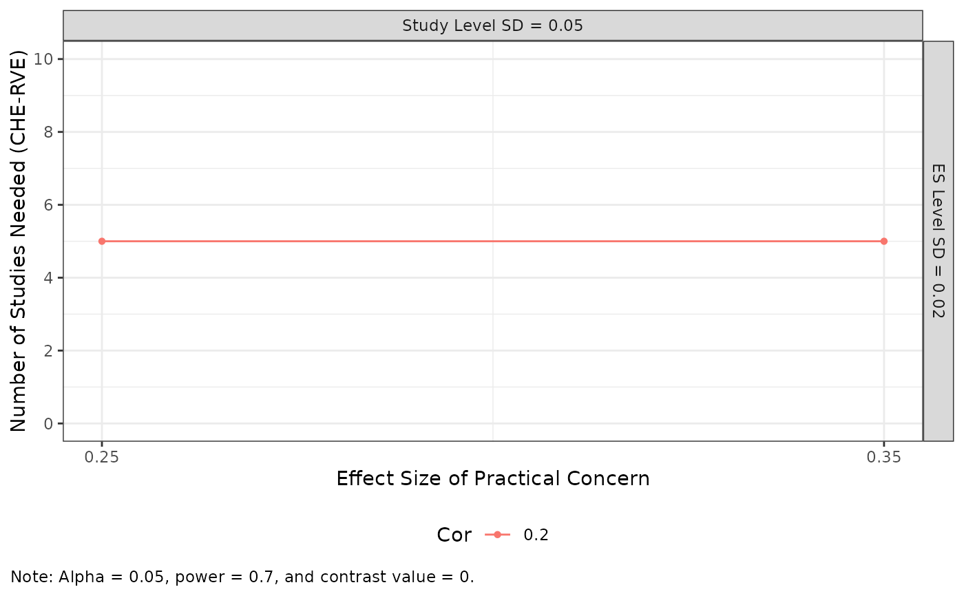
Value
A ggplot plot showing the minimum number of studies needed to
obtain a given effect size with a certain amount of power and level-alpha, faceted
across levels of the within-study SD and the between-study SD,
with different colors, lines, and shapes corresponding to different values
of the assumed sample correlation. If length(unique(data$mu)) > 1, it
returns a ggplot plot showing the minimum studies needed
to obtained a given effect size with a certain amount of power and
level-alpha across effect sizes of practical concern, faceted by the
between-study and within-study SDs, with different colors, lines, and
shapes corresponding to different values of the assumed sample correlation.
Details
In general, it can be rather difficult to guess/approximate the true
model parameters and sample characteristics a priori. Calculating the
minimum number of studies needed under just a single set of assumptions can
easily be misleading even if the true model and data structure only
slightly diverge from the yielded data and model assumptions. To maximize
the informativeness of the analysis, Vembye, Pustejovsky, &
Pigott (In preparation) suggest accommodating the uncertainty of the power
approximations by reporting or plotting power estimates across a range of
possible scenarios, which can be done using plot_MADE.power.
References
Vembye, M. H., Pustejovsky, J. E., & Pigott, T. D. (In preparation). Conducting power analysis for meta-analysis of dependent effect sizes: Common guidelines and an introduction to the POMADE R package.
Examples
min_studies_MADE(
  mu = c(0.25, 0.35),
  tau = 0.05,
  omega = 0.02,
  rho = 0.2,
  target_power = .7,
  sigma2_dist = 4 / 200,
  n_ES_dist = 6,
  seed = 10052510
) |>
  plot_MADE(y_breaks = seq(0, 10, 2), numbers = FALSE)
#> Warning: Notice: It is generally recommended not to draw on balanced assumptions regarding the study precision (sigma2js) or the number of effect sizes per study (kjs). See Figures 2A and 2B in Vembye, Pustejovsky, and Pigott (2022).